Linear Regression: Two Solvers and the Checks After Fitting
Linear regression is easy to fit and easy to misuse. Its coefficients can describe how an expected outcome changes with the input variables, but only after the observation unit, feature timing, and model assumptions have been made explicit.
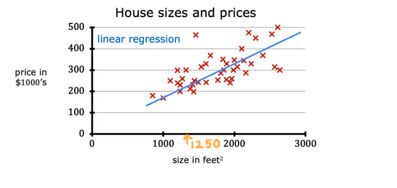
One model, from one feature to polynomial features
-
One input variable:
y = w*x + b
-
Multiple input variables:
y = w1x1 + w2x2 + … + wn*xn + b
-
Polynomial terms treated as engineered input features:
y = w1x1 + w2x1^2 + … + b
Use it for prediction or for understanding relationships
- Predict a continuous output such as house price, stock value, or credit score.
- Examine a relationship, such as whether a higher interest rate is associated with a higher total savings-book balance.
These goals are not interchangeable. A model can predict well while individual coefficients remain unstable, and a coefficient that describes an association does not prove that changing the feature will cause the outcome to change. In the savings example, customer characteristics may influence both the offered interest rate and the balance.
Before fitting, define one row and one cutoff date. If one row represents one customer at month-end, every predictor must be available by that month-end and the target must belong to the intended future or contemporaneous window. This prevents information from the target period from leaking into the features.
Fit the same model in two ways
Given x and y, the coefficients can be estimated iteratively with gradient descent or directly with matrix operations. Implementing both makes the difference between optimization and a closed-form solution concrete.
- Gradient descent: iteratively reduces the loss and exposes the role of learning rate, feature scale, and convergence.
- Matrix solution: calculates the least-squares coefficients directly and exposes the role of matrix rank and collinearity.
Both approaches estimate the same linear model. They differ in computation, not in the relationship being assumed between the predictors and outcome.
Gradient descent updates the slope and intercept iteratively
Step 1: Initialize w and b
# initialize w

w_init = -0.01
w_init

# initialize b

b_init = 46
b_init

learning_rate = 0.0000001
loss_history = []
w_history = []
b_history = []
Step 2: Calculate mean squared error
def calculate_mse(y_pred, y):
    mse = 0
    for i in range(len(y)):
        mse += ((y_pred[i] - y[i])**2)/len(y)

    return mse
Step 3: Calculate the gradients
def grad_y_by_w(w, b, x, y):
    tot_grad = 0
    for ele in range(len(x)):
        tot_grad += (1/len(x))*(w*x[ele] + b - y[ele])*x[ele]
    return tot_grad

def grad_y_by_b(w, b, x, y):
    tot_grad = 0
    for ele in range(len(x)):
        tot_grad += (1/len(x))*(w*x[ele] + b - y[ele])
    return tot_grad
Step 4: Update w and b over multiple epochs
for epoch in range(30):
    print("================================")
    print(f"Run for epoch {epoch}")

    if epoch == 0:
        w = w_init
        b = b_init
        y_pred = w*x + b

    if epoch >= 1:
        grad_l_by_w = grad_y_by_w(w, b, x, y)
        grad_l_by_b = grad_y_by_b(w, b, x, y)
        print(grad_l_by_w)
        print(grad_l_by_b)

        w = w - learning_rate*grad_l_by_w
        b = b - learning_rate*grad_l_by_b

        print("w: ", w)
        print("b: ", b)

        y_pred = w*x + b


    loss = calculate_mse(y_pred, y)
    # print(loss)
    loss_history.append(loss)
    print("Loss: ", loss)
    w_history.append(w)
    b_history.append(b)
Step 5: Compare with scikit-learn
import numpy as np
from sklearn.linear_model import LinearRegression, SGDRegressor

# data
X = np.array([[1], [2], [3], [4], [5]], dtype=float)
y = np.array([1.2, 1.9, 3.2, 3.9, 5.1])

# exact OLS
lr = LinearRegression().fit(X, y)
print("LinearRegression coef:", lr.coef_, "intercept:", lr.intercept_)

# gradient descent version
sgd = SGDRegressor(max_iter=10000, eta0=0.01, learning_rate='constant').fit(X, y)
print("SGDRegressor coef:", sgd.coef_, "intercept:", sgd.intercept_)
Matrix operations give a direct solution
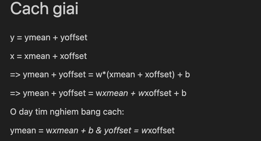
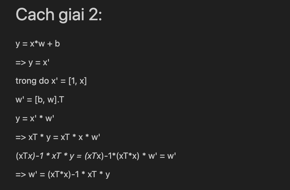
The following notebook snippets calculate the intercept and slope from the design matrix and from centered variables.
n = len(x)
x_temp = np.concatenate([np.ones((n, 1)), np.reshape(x, (n,1))], axis=1)

x_temp

w_temp = np.linalg.inv((x_temp.T) @ x_temp) @ (x_temp.T) @ y

w_temp

b = w_temp[0]
w = w_temp[1]
ymean = y.mean()

xmean = x.mean()

ymean

yoffset = y - ymean
xoffset = x - xmean

yoffset

w = (xoffset.T @ yoffset) / (xoffset.T @ xoffset)

w

b = ymean - xmean*w
b
The first form follows the normal equation directly. In production code, np.linalg.lstsq is preferable to explicitly calculating a matrix inverse, especially when predictors are close to linearly dependent.
The closed-form expression is useful for understanding the estimator, but explicitly forming an inverse adds numerical risk and unnecessary work. Gradient descent avoids that inverse, although it introduces a learning rate, stopping rule, and sensitivity to feature scale.
Benchmark iterative and direct solvers
import time
import numpy as np
from sklearn.linear_model import LinearRegression, SGDRegressor

def benchmark(n_samples, n_features):
    X = np.random.randn(n_samples, n_features)
    y = np.random.randn(n_samples)

    # LinearRegression
    start = time.time()
    try:
        LinearRegression().fit(X, y)
        lr_time = time.time() - start
    except Exception as e:
        lr_time = str(e)

    # SGDRegressor
    start = time.time()
    SGDRegressor(max_iter=1000).fit(X, y)
    sgd_time = time.time() - start

    return lr_time, sgd_time

sizes = [(1000, 1000), (2000, 2000), (5000, 5000), (10000, 1000), (1000, 10000)]
for n, d in sizes:
    print(f"n={n}, d={d}:", benchmark(n, d))
The larger cases in this benchmark allocate dense matrices and can require substantial memory; they should be run individually rather than treated as a lightweight example.
A fair comparison records more than elapsed time. It should use the same generated data, compare coefficient or prediction error, and report whether either solver failed because of memory, convergence, or an ill-conditioned design matrix. A faster answer is not useful if it is numerically different from the least-squares solution.
Check the assumptions after fitting
The fitted coefficients and predictions are not the end of the analysis. The residuals help show whether the linear model is a reasonable description of the data.
The importance of each assumption depends on the goal. Normal residuals are mainly relevant to small-sample inference; they are not a requirement for calculating least-squares predictions. Linearity, leakage, changing variance, dependent observations, and influential points can damage the model even when a normality test looks acceptable.
| Assumption | How to check it | Tool |
|---|---|---|
| Linearity | Plot residuals against fitted values | sns.residplot() |
| Independent errors | Check serial correlation; Durbin–Watson is useful for ordered or time-series data | durbin_watson() |
| Constant variance | Inspect residuals versus fitted values or run a Breusch–Pagan test | statsmodels |
| Approximately normal residuals | Use a Q–Q plot, histogram, or Shapiro–Wilk test | shapiro(), qqplot() |
| No severe multicollinearity | Calculate the Variance Inflation Factor | variance_inflation_factor() |
Residual plots diagnose patterns left by the fitted model; they do not prove that the data-generating assumptions are true. Independence in particular comes mainly from the sampling and time structure. A Durbin–Watson statistic cannot repair duplicated customers, overlapping time windows, or another dependence introduced during dataset construction.
Inspect the residual distribution visually
For the Shapiro–Wilk test:
H₀: the residuals follow a normal distribution.- If
p < 0.05, rejectH₀.
With a large sample, even a small departure from normality can produce a very small p-value. A Q–Q plot and histogram show whether that departure is material rather than merely detectable.
Q–Q plot:
import statsmodels.api as sm
import matplotlib.pyplot as plt

sm.qqplot(np.array(resid), line='45', fit=True)
plt.show()
Histogram:
import seaborn as sns
import matplotlib.pyplot as plt

sns.histplot(resid, kde=True)
plt.show()
VIF exposes predictors that repeat the same information
To calculate the VIF for feature Xᵢ, regress it on the remaining predictors and use the resulting Rᵢ²:
VIF_i = 1 / (1 - R_i²)
A VIF above 5 corresponds to Rᵢ² > 0.8 and is a signal to inspect the feature. It is a diagnostic threshold, not an automatic instruction to delete the variable.
import pandas as pd
from statsmodels.stats.outliers_influence import variance_inflation_factor
from statsmodels.tools.tools import add_constant

# X is a DataFrame containing the predictors
X = add_constant(x)

vif_data = pd.DataFrame()
vif_data["feature"] = X.columns
vif_data["VIF"] = [variance_inflation_factor(X.values, i) for i in range(X.shape[1])]

print(vif_data)

Three responses to multicollinearity
When several predictors carry overlapping information, there are three practical options:
- Remove predictors that duplicate information already represented elsewhere.
- Combine correlated predictors, for example with Principal Component Analysis.
- Use regularization such as Ridge or Lasso.
The choice depends on the goal. Removing or combining features changes interpretation; regularization keeps the model predictive while shrinking unstable coefficients.
For explanation, removing a redundant feature may preserve a coefficient that the business can still interpret. For prediction, Ridge often keeps correlated signals without forcing an arbitrary winner. PCA can reduce dimension but replaces named business variables with linear combinations. Lasso performs selection through shrinkage, yet among strongly correlated predictors the selected variable can change across samples.
PCA keeps directions with the most variance
For a square matrix A, an eigenvector v and eigenvalue λ satisfy:
Av = λv
Multiplying v by A changes its scale by λ without changing its direction.
In PCA, A is the covariance matrix. Each eigenvalue measures how much variance is retained along its corresponding eigenvector. Sorting eigenvalues from largest to smallest ranks the principal-component directions by the information they retain.
The explained-variance ratio is used to select the first k components—for example, enough components to retain 95% of the variance.
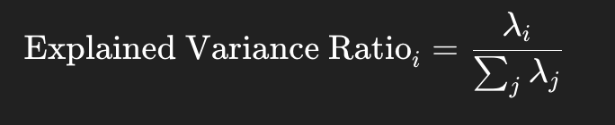
An n × n covariance matrix has n eigenvalue–eigenvector pairs:

Placing the selected eigenvectors into a projection matrix transforms the original m features into k principal components. This reduces dimension, but the new components are combinations of the original variables and are therefore less direct to interpret.
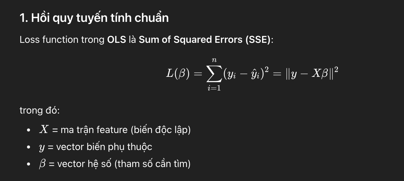
Ridge and Lasso keep the predictors but penalize coefficients
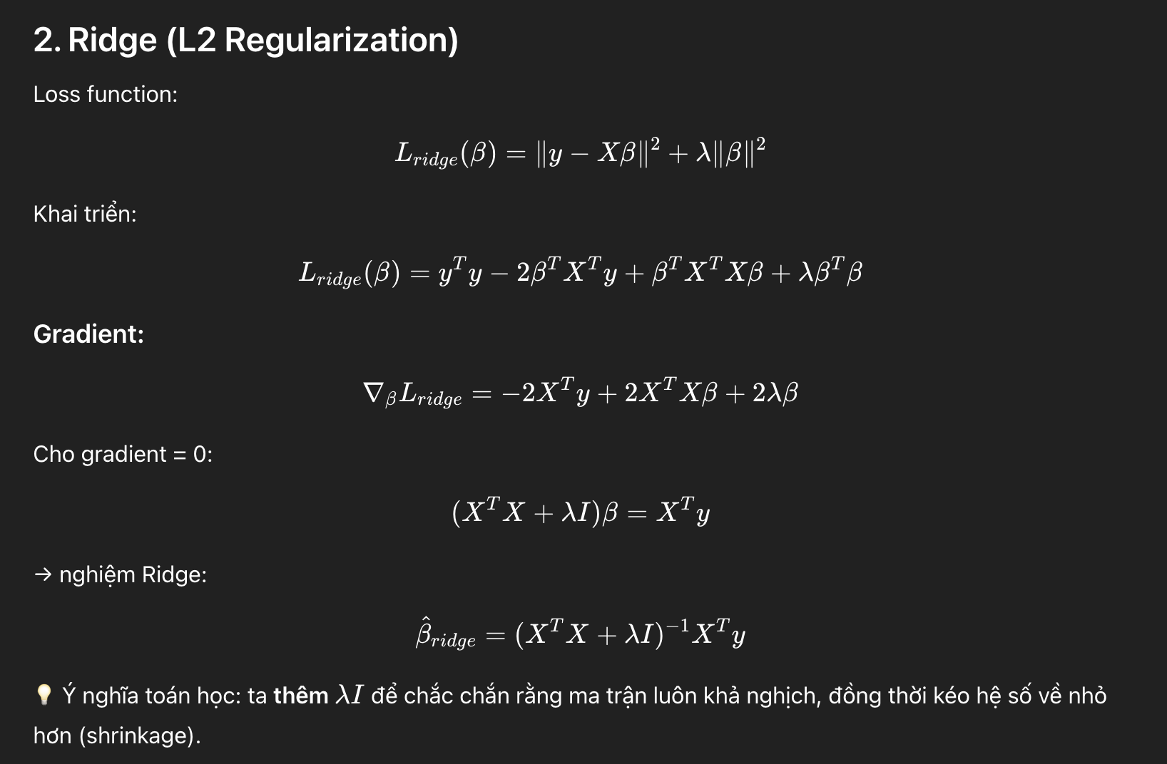
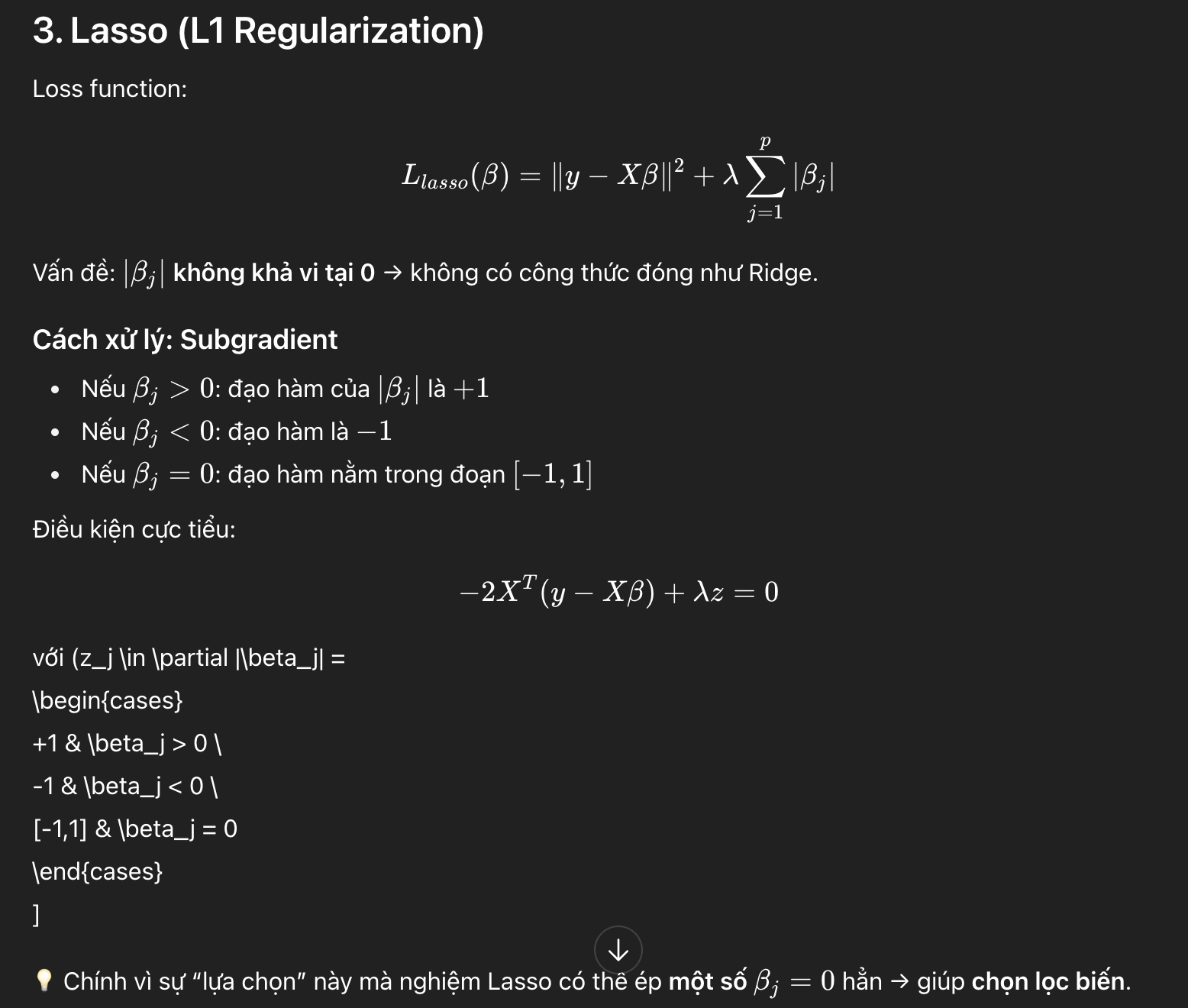
Ridge adds an L2 penalty and shrinks correlated coefficients. Lasso adds an L1 penalty and can reduce some coefficients to exactly zero.

Ridge solution

Lasso solution
Choose the response to match the failure
| Observed problem | First response to consider |
|---|---|
| Curved residual pattern | Add justified nonlinear structure or change the model |
| Variance grows with fitted value | Revisit the target scale or use inference robust to heteroscedasticity |
| Serially correlated errors | Model the time or group dependence explicitly |
| High VIF but prediction remains stable | Prefer regularization if prediction is the goal |
| High VIF and coefficients must be explained | Remove, combine, or redefine overlapping features |
| A few rows control the fitted line | Inspect influential observations and the data-generation process |
The solver answers how to estimate the coefficients. Residual checks, validation data, and the intended use of those coefficients answer whether the fitted model deserves to be used.