Decision Trees: How a Split Is Chosen
At each node, a decision tree has one job: choose the feature and threshold that separate the target classes most clearly. Understanding that search explains both how the tree learns and why an unrestricted tree can overfit.
Reference: Machine Learning Cơ Bản — Decision Tree
Search every feature for a useful threshold
For each numerical feature, the basic algorithm:
- Sorts the observed values.
- Places candidate thresholds between consecutive distinct values.
- Splits the rows into left and right child nodes at each threshold.
- Calculates the impurity after the split.
- Chooses the feature and threshold with the largest impurity reduction.
If a feature has n distinct values, it has at most n - 1 candidate thresholds.
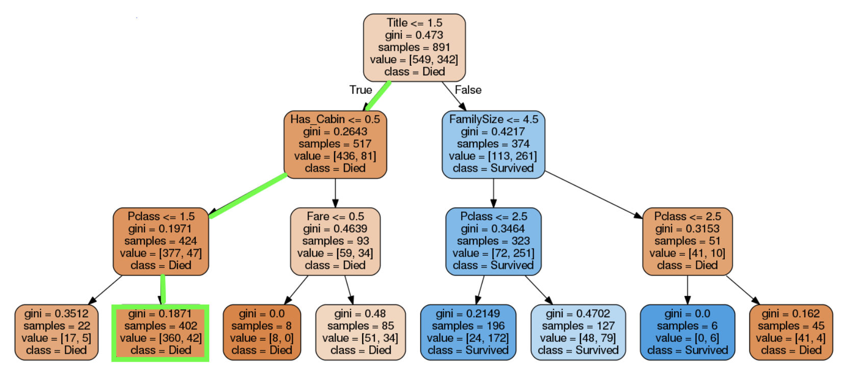
Lower Gini means cleaner child nodes
For a classification node, Gini impurity is:
Gini = 1 - Σ p(k)²
If both classes are mixed 50/50 in a child node:
Gini = 1 - 0.5² - 0.5² = 0.50
Suppose another split produces class proportions of 0.3/0.7 on the left and 0.8/0.2 on the right:
- Left Gini:
1 - 0.3² - 0.7² = 0.42 - Right Gini:
1 - 0.8² - 0.2² = 0.32
When the two child nodes contain the same number of rows, their weighted impurity is (0.42 + 0.32) / 2 = 0.37, lower than 0.50. If the child sizes differ, their Gini values must be weighted by their number of rows before comparing splits.
For example, start with 10 rows split evenly between two classes, so the parent Gini is 0.50. A candidate threshold creates:
- A left child with 3 rows from Class A and 1 from Class B:
Gini_left = 0.375. - A right child with 2 rows from Class A and 4 from Class B:
Gini_right ≈ 0.444.
The child sizes are different, so the post-split impurity is:
(4 / 10) × 0.375 + (6 / 10) × 0.444 ≈ 0.417
The impurity reduction is approximately 0.50 - 0.417 = 0.083. This gain—not the Gini of either child by itself—is what makes the candidate comparable with another split.
Entropy or log loss can be used instead of Gini, but the decision remains the same: prefer the split that reduces impurity the most.
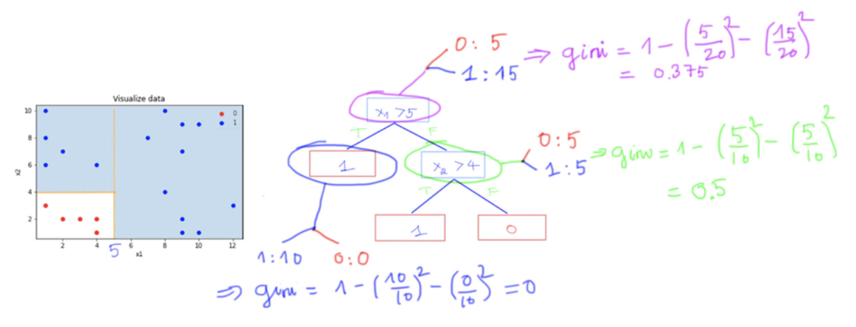
Exhaustive search does not mean testing arbitrary numbers
For a continuous feature, there is no reason to test every real number. Only boundaries between consecutive observed values can change which rows fall into the left and right nodes. Tree implementations exploit this fact instead of testing arbitrary thresholds.
The search can be reduced further in practice:
max_featuresrestricts the number of features considered at a node.splitter="random"samples candidate thresholds instead of always selecting the best one.- Histogram-based or approximate tree algorithms group continuous values into bins.
- Compiled implementations such as scikit-learn’s Cython tree code avoid Python-loop overhead.
Scikit-learn’s standard decision trees do not handle categorical features natively. Integer-encoding a category makes the values look ordered, so the resulting numeric thresholds may not represent meaningful category groups.
For a category such as acquisition channel, codes 1, 2, and 3 do not imply a real ordering. A rule such as channel_code <= 1.5 is therefore an artifact of the encoding unless that ordering was intentionally defined. One-hot encoding avoids the false order, but it changes the available partitions and can widen the feature space.
Stopping rules control how much the tree memorizes
Even a useful split may create leaves that are too specific to the training data. The main controls are:
max_depth: maximum number of levels.min_samples_split: minimum rows required before a node can split.min_samples_leaf: minimum rows that must remain in each child.max_features: features considered at each split.
The split criterion explains how the tree grows. These stopping rules determine when it should stop.
Lower training impurity does not mean a better tree
If growth is unrestricted, the tree can keep creating leaves that explain smaller and smaller groups of training rows. Training impurity falls, but the rules become fragile and may not generalize.
The stopping parameters should be selected with validation data or cross-validation rather than by inspecting training accuracy. Cost-complexity pruning provides another route: grow a larger tree, then penalize additional leaves and select the subtree that gives the best validation trade-off.
The final tree should be inspected as a set of rules. A split that uses a suspicious identifier, a post-outcome field, or a category code with no real order may look statistically useful while revealing leakage or bad feature design.
Understanding Gini explains how a candidate split wins. Validation and pruning answer the separate question that matters in practice: whether the resulting rule will work on new observations.